Contour Method at the University of Manchester

Resources for using the Contour Method to determine residual stress

• Home
• Resources

Contents

CMM methodology for contour method measurements
Using the Mitutoyo Crysta-Apex 776 as a surface profilometer

1 Introduction

The following documents the latest techniques for capturing surface profiles with the CMM for use in the contour method. First, previous approaches will be covered, followed by new techniques to address some of the shortcomings of these prior approaches. Pursuant to this, the main topics covered will be:

• Orientation of the specimen on the CMM and baseline measurements required to account for self-restraint features
• Segmentation and targeting point measurement locations
• Meshing and writing the point measurements to a format which can be interpreted by the ASCII-GEOPAK converter
• Previewing results

This will covered using a NeT TG6 specimen as an example.

1.1 Background

The first contour method surface measurements were conducted using a coordinate measurement machine [1]. When using a CMM, it has been shown that using a point measurement scheme is a more accurate means of measuring surface variations on a contour-cut surface as opposed to using a probe-dragging technique after Johnson[2]. Johnson referred to this latter technique as ‘continuous’ probe movement, and noted that intermittent contact or ‘hen-peck’ mode was more accurate due to the controlled approach trajectory of the probe tip.

The literature indicates that the point spacing required to adequately capture the surface is between 30-250 $\mu$m, depending on the stress gradient changes along the cut surface. The practical issue is then how to target regions of interest with adequate point density with the CMM programming practices at the analyst’s disposal. The manner which has been devised previously is to use the stylus-drag technique on the periphery of the component to generate a closed polygon or hull and then populating the interior with programmed point locations.

1.2 Methodology

Using a standard Cartesian coordinate system with the $z$ axis normal to the mean contour cut surface, the probe is programmed to capture the cross-section of the component at some proscribed $z$ value just below the cut plane. This is accomplished by dragging the probe around the component with a constant deflection and recording $x$ vs. $y$ data of the outline with a proscribed discrete pitch as recorded at the probe’s centre. The recorded path captured directly by the position encoders is then offset by the probe’s radius to arrive at the contour on the surface of the component.

It then remains to decide on how to best populate this outline with surface measurement points adequate both in number and distribution. Johnson employed a brute-force technique, which first took the $xy$ Cartesian extents of the hull obtained in the manner described above, and then devised a very fine rectilinear grid of points encompassing these extents as measurement points. Points of this grid contained within the hull were then identified (Fig. 1).

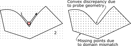
While this is an acceptable technique where components with a predominantly rectilinear cross-section are considered, there are some issues worth noting:

• For cross-sections which are not rectilinear, points close to non-orthogonal edges are lost. The overall grid density has to be increased appreciably in order to get points closer to the edges. This is an issue if there is large variation in the cross-section along $z$, and the outline captured may not reflect the edges at the cut surface.
• Surface measurements of points very close to the component edges are included. In the case of components that contain convex regions with high entry angles, the apparent outline will be captured to appear larger than it actually is owed to the probe diameter. This can result in a point which is not on the component’s cut surface. This discrepancy is normally quite small with an adequately small enough probe diameter.

The current methodology consists of capturing the outline as described above, negatively offsetting the outline by a small amount, and then meshing the result. The nodes of the mesh are then used as measurement points (Fig. 2).

This approach addresses some of the issues identified above. First, by negatively offsetting the hull, the analyst can be sure that any points within this domain actually lie on the contour cut surface. Second, using meshing techniques is a more efficient use of measurement points. Curvature can be better captured, and point density can be varied depending on the stress gradient expected using mesh refinement techniques.

This methodology is described subsequently using a NeT TG6 specimen and the techniques demonstrated can be extended to any variety of contour method specimens.

2 Orientation and baseline measurements

For most contour measurements, the most facile orientation of the specimen is to align the cut surface such that the normal of the mean plane of the cut face is directed along the positive $z$ axis of the CMM.

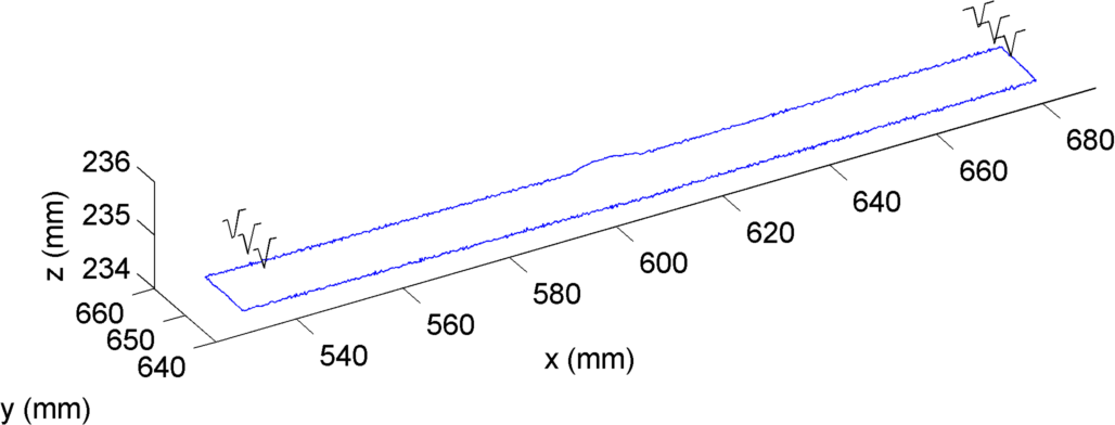
This can be accomplished by any number of ways, just as long as the specimen is held firmly so that it does not move during measurement, but not with enough force to deform the sample. Fig. 3 shows the typical orientation of a bead-on-plate weld specimen. This specimen first had two electro-discharge machined holes placed on either side of the specimen’s region of interest. A contour cut was then performed between these two holes, with the ligaments on either side of the hole acting as self-restraint features during cutting. Once the contour cut was performed, each of these ligaments were cut to provide access for contour measurements. This creates a surface which is punctuated by semi-cylindrical features which need to be captured for accurate contour method analysis.

In order to populate the methods used to place contour method points, 7 contours in total will need to be captured using the SCANPAK functionality on the CMM. First, the $xy$ outline will be captured, followed by 6 scans of the self-restraint features. These are shown in Fig. 4 and 5.

It is important when setting up that the contour cut surface is not grossly misaligned with the principle CMM axes, particularly in the $z$ direction; i.e. ‘Angular misalignment’ as shown in Fig. 5 is minimized. The orientation of the cut surface should reflect the cutting direction along the $x$ axis. It is important that the line scans are conducted in the following sequence, and each of the seven scans are saved to independent text files:

• The $xy$ outline trace should start from the far left of the component, mid-way along the $y$ extents of the outline, and then trace out the contour in a clockwise fashion. Depending on the size of the part, a pitch of 50-100 $\mu$m is advised.
• While the order in which the six $xz$ traces are performed on the CMM is not critical, the order in which they are further processed is important so for the sake of convenience perform the $xz$ traces in the order shown in Fig. 5. Traces 1-3 and 4-6 should be spread out approximately equidistantly vertically along $y$, with traces 1, 3, 4, and 6 placed close to the $xy$ cross-section boundary.
• The $xz$ traces are conducted by bringing the probe to approach the surface along the $-z$ direction, approximately 1 mm away from the $-x$ edge of the self restraint feature, carried across the surface to 1 mm past the restraint feature. A pitch of $<50$ $\mu$m should be employed for these traces.

At this point, the points collected with the CMM should appear as shown in Fig. 6.

3 Segmenting the outline

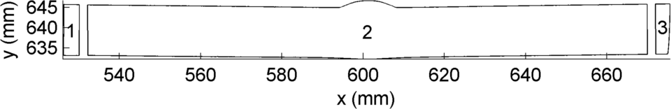
Once the traces have been captured, information contained within is used to calculate ‘islands’ making up the overall surface. At this stage in the analysis, the semi-cylindrical self-restraint regions will be isolated such that three discrete regions, described by independent $xy$ hulls are obtained to populate with CMM point measurements.

A script called OutlineGen.m has been provided for this purpose. The script performs the following steps:

1. Reads in the seven profiles obtained in the previous step, which are placed in a cell structure according to the sequence $x{z}_1,x{z}_2\dots x{z}_6,xy$ where $x{z}_n$ is the sequence described in Fig. 4.
2. Passes the maximum $z$ value in the $xz$ series of scans to zmax.
3. Working from the origin, identifies the edges of the self-restraint features as they appear along the $x$ axis by from the $xz$ scans by:
   1. Identifying the first and last points along each trace where $dx∕dz>0.05$ then
   2. Fitting a line to the three points identified on each edge as a result using linefit.m.
4. Uses poly2poly.m (Bruno Long, 2010), to solve for the intersection points of the lines identified by linefit.m and the $xy$ outline.
5. Segments the $xy$ outline according to these intersection points.
6. Writes each of the three segments of the $xy$ profile and zmax to a ⋆.mat file corresponding to the prefix of the $xy$ outline file containing a cell structure outline which contains three fields for each segment. The first entry in outline has the lowest $x$ value, the second is the region between the two restraint features, and the third is the remaining outline, as per Fig. 7.

4 Meshing and writing points to a measurement file

Now that the outline has been segmented, points to have the CMM measure from in the $xy$ can be identified. This is done by meshing each segment of the outline using an appropriate meshing engine.

A utility has been provided to do so, MeshMeas.m. This script does the following:

1. Clears the workspace, and initializes local directories as to where part programs, result files and outline files are stored. If this is the first time running the program, the boolean redo variable should be set to false. Mesh refinement and location can be specified here.
2. The two main inputs required are where the ASCII code will be stored, the file name/location of where the measured points are intended to go, and the name of the program as it will appear in GEOPAK/MCOSMOS. Note that the measurement file requires an absolute path, GetFullPath.m (Jan Simon 2013) is used to generate the appropriate string from a relative path.
3. If the appropriate flag is set, read in an intermediate mesh file. Otherwise go through with meshing it, starting with reading the outline file.
4. Loops through the outlines and performs the following on each outline:
   1. Offsets the outline by xyOff using Clipper (Angus Johnson 2014). A MATLAB function wrapper for Clipper has been provided for Matlab running under 64-bit Windows 7, called clipper.mexw64.
   2. The coordinates of the polygon representing the offset outline is then re-spaced equally according to the seed spacing along the path integral using respace_equally.m.
   3. For each offset outline it creates a 2D mesh using a modified version of distmesh2d (Per-Olof Persson 2012) with a characteristic seed spacing. The modified distmesh2d function has been provided, but relies on the distmesh v1.1 library being on the MATLAB path at the time of running MeshMeas.m. If mesh refinement is selected, then the second outline will be refined, either along the mean of the $x$ coordinates by default, or at user-specified $x$ and $y$ locations. Otherwise, distmesh2d will attempt to render an evenly distributed mesh. Mesh retriangulation has been limited to 1000 iterations, permitting relatively large but potentially imperfect meshes to be generated in a reasonable amount of time. See Section 4.1 for more information.
5. After the mesh is complete, then a MeshIntermediate.mat file will be generated containing the following as cell structures, with each cell entry corresponding to an outline in the sequence described in Fig. 6:
   • The starting outline
   • The perimeter of the starting outline
   • Nodes
   • Node connectivity
6. Once the mesh has been created, then the nodes from the mesh, a $z$ coordinate to start measuring the surface from, and paths/file names are passed to meshgen_cmmpnts.m which writes the program to be interpreted by GEOPAK/MCOSMOS. See Section 4.2 for more information on this utility.

4.1 Meshing

A uniformly-distributed mesh without refinement places points evenly across the outline of the component (Fig. 8). This is obtained in MeshMeas.m by setting the refine variable to an empty vector i.e. refine=[].

There are a number of pre-defined methods for creating a distributed mesh. Ideally, a higher density of points should be placed in regions with potentially high stress gradients. For the NeT TG6 specimen and other other weld validation coupons with similar geometries, this includes regions around the heat affected zone. By setting the refine variable to zero i.e. refine=0, the mesh will be refined across the mean $x$ coordinate of the second outline (Fig. 9). The mesh will range from the proscribed seed spacing to half of this at the points specified by refinement.

For refinement at an arbitrary location, then a polyline can be specified by entering an $N\times 2$ matrix for the refine variable. Fig. 10 shows the result when refine=[574.9 638.6; 590.8 637.2]. Multiple further points describing a linearized boundary of the fusion zone, for example, can be added.

The rate of change of the mesh is specified by a minimization function appearing as:

fh=@(p) min(P/2+P⋆0.01⋆abs(dpoly(p,tp)),P);}

where P is the seed spacing, p is the nodes and tp are the refinement points. The constant 0.01 defines the rate of change of refinement as tp is approached from the outside edges. It is not recommended that this value is changed unless the domain warrants it.

Dismesh is not a particularly fast mesh generator. The user should be aware that meshing with distmesh2D.m gets slower exponentially with the number of nodes requested. For example, a recent run requesting 19k points required nearly an hour to complete. As the contour method moves to open source, GMSH will be integrated.

4.2 Generating a part programme

Programming the CMM usually takes the form of peforming measurements in ‘Learn’ mode. There are other Mitutoyo modules which can accept components in various CAD formats and a measurment regime can be programmed graphically. Early CMM programmers used a text-based programming language based loosely on RS-274 (G-code) called the Dimensional Measuring Interface Standard (DMIS). While many smaller CMM manufacturers rely on a version of DMIS for CMM programming, Mitutoyo provides only limited support for DMIS-type commands in the form of the ASCII-GEOPAK converter. It is worth mentioning that there is also currently the possibility of exporting GEOPAK programmes to DMIS-type ASCII-based commands, but is beyond the scope of this guide.

A DMIS-like program is written by a call to meshgen_cmmpnts.m within MeshMeas.m. The function meshgen_cmmpnts.m is called by

meshgen_cmmpnts(zmax+1.5,PPgm,GPakFName,MeasFile,p,'new')

where zmax is the maximum $z$ value or highest point on the surface, PPgm is the relative path and prefix of ⋆.agw where the ASCII programme will be written, GPakFName is the programme name that will appear in the MCOSMOS part manager, MeasFile is the absolute path and file name of where the measurement results will go, p is an $N\times 2$ matrix of $x$, $y$ node coordinates created by meshing and ‘new' is an unused status flag. This function does the following:

1. Writes a file name to be interpreted by GEOPAK (GPakFName). This is the programme name that will appear in the MCOSMOS part manager.
2. Selects what appears as probe 1 in GEOPAK. Upon executing this line, the probe will change if it is not in the probe 1 position.
3. Initializes the machine by turning on computer numeric control with default movement and measurement speeds.
4. Creates a contour scan object.
5. Writes measurement and position variables, ZCLEAR and ZMEASUREMENT. ZCLEAR will be written as the maximum $z$ value found from the $xz$ traces plus 100 mm. ZMEASUREMENT will be written as the maximum $z$ value found from the $xz$ traces plus 1.5 mm. This latter value is written by the zmax+1.5 argument in the meshgen_cmmpnts.m call.


It is the users responsibility to ensure that the value recorded when tracing the restraint features in the $xz$ plane reflects the maximum $z$ value. Otherwise, a crash can result.

6. From wherever the probe is currently located, moves the probe to ZCLEAR along the $z$ axis.
7. Moves the probe in 3 directions to the $x$, $y$ position of node 1 in the mesh of the first outline and $z=$ZMEASUREMENT. Enters measurement mode, and approaches the surface in the $-z$ direction.
8. Repeats this for the next 99 points to form a block, completes the contour scan object and then exports the values for each point contained therein to a newly created measurement file. If this file exists, it is overwritten.
9. Repeats the above, but for the next and subsequent blocks, the results are appended to the file created/overwritten in the previous step.
10. Writes an end of measurement flag.
11. Writes an end of file flag, with a carriage return after.

This programme works the best if execution is started with the machine having probe 1 set to A=0º, B=0º and in place and close to the home position. The programme will complete with the probe located at the last $x$,$y$ point $z=$ZMEASUREMENT.

In order to convert the generated ⋆.agw file into a GEOPAK-interpreted programme, start MCOSMOS. From the part manager screen (Fig. 11), access the ASCII-GEOPAK conversion utility via CMM $▹$ ASCII-GEOPAK Converter. To convert, select File in the utility (Fig. 12) and navigate to where the ⋆.agw is located. The programme will appear under programme list in the part manager. This programme can be run as any other GEOPAK programme, and can be previewed by selecting CMM $▹$ Part Program Editor from the MCOSMOS part manager screen.

5 Previewing results

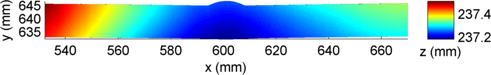
Prior to removing the specimen, it is important to preview the results to ascertain whether or not points will need to be remeasured, whether all points specified were indeed measured, etcetera. A simple scatter plot function has been provided for such a purpose, ResultPreview.m. This function is called by

ResultPreview('ResultDirectory\MeasurementFile.txt')

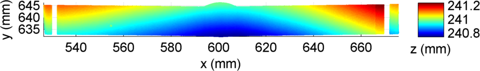
where the argument is either a relative path to where the function is being called or an absolute path, and the text file created by the measurement programme. Output is a plot similar to Fig. 13.

In order to extract only the central section of the surface i.e. the surface between the restraint features the inpoly.m (Darren Engwirda, 2007) function can be employed. The inpoly.m function is an optimized version of MATLAB’s inpolygon.m. For example, running dlmread.m on the results file and passing the resulting $N\times 3$ to a variable P and loading the outline ⋆.mat generated by OutlineGen.m:

P=dlmread('ResultDirectory\MeasurementFile.txt');
load('OutlineGenDirectory\Discretized_1.mat');
in=inpoly(P(:,1:2),outline{2}(:,1:2));
x=P(in,1); y=P(in,2); z=P(in,3);

will return all points contained in the central outline to x, y and z. A scatter plot of x, y and z is shown in Fig. 14.

6 Summary

This concludes the guide on how to generate contour method surface measurements with the Mitutoyo CMM. All scripts described have been included in the stress analysis code repository in the CMM directory including:

• OutlineGen.m, including dependent functions:
  • linefit.m
  • poly2poly.m
• MeshMeas.m, including dependent functions:
  • GetFullPath.m
  • clipper.mexw64
  • respace_equally.m
  • The modified distmesh2d.m function, but not the dependent functions from the distmesh library. Note that the distmesh library contains a distmesh2d.m function, but placing the modified version on MATLAB’s work path will supersede it.
  • meshgen_cmmpnts.m
• The function ResultPreview.m

Note that inpoly.m is already located in the Utils folder of the code repository.

While every effort has been made to ensure the scripts work as intended with MATLAB R2013a (v8.1.0.604), this code is distributed without warranty. If issues arise, please generate a minimum working example of the bug, document steps taken to address it and email it to the contour method listserv.

References