Mitutoyo Crysta-Apex 776 user guide:
Basic instruction
This guide is partially based on a guide originally written by Joanna Walsh and Nick O'meara. It was expanded upon to include specific details and operating procedures for an older version of MCOSMOS. MCOSMOS has since been upgraded and many of the GUI and menu options details have changed location slightly. This guide is intended to be used in a procedural capacity only until it is updated to reflect the new software.
1 Introduction
This document is intended as an introduction and reference guide for new users of the Mitutoyo Crysta-Apex 776 Coordinate Measurement Machine (CMM). The machine will be first introduced with the main features described, which will be followed by a start-up and shut-down sequence instruction. This will be followed by a description of how to perform basic probe setup and calibration. Finally, instruction on how to run a single line scan will be discussed.
1.1 Machine overview
The CMM is a powerful tool for part digitization and metrology. Measurements are gathered by various probes which are moved into position either manually or by computer control. These probes may be optical (non-contact) or mechanical (contact); readings from these probes are then translated into either unregistered points or geometric constructs depending on the software interpretation of the data. Since the measurement of these points may be automated without operator intervention, a CMM is a specialized form of industrial robot. As such, all of the precautions that are associated with automated equipment should be adhered to, particularly during maintenance, setup or adjustment. Operator injury is a primary concern, but an immediate second concern is prevention of damage to the probes which are both high-precision and value instruments.
Most CMMs follow similar designs: a high precision Computer Numeric Control (CNC) series of axes which is built on a precision bed. The probe is fixed to a single point on a ‘bridge’ which spans the bed, and the bridge traverses the bed. These working axes are in the direction across the bridge, the direction longitudinally along the bed and which runs vertically from the bridge. In order to maintain a high degree of accuracy over large travel distances, friction and lash on the active axes is limited through the use of air-bearings. As a result, the CMM requires a constant supply of pressurized air free of dust, oil and moisture and control circuitry should be protected from power surges.
1.1.1 General machine layout
Fig. 1 shows the general layout of the Crysta-Apex. Located on the front of the machine, there is a series of air filters designed to pull trace amounts of oil and water from the air supply, along with a valve and a pressure sensor/switch (Fig. 1). The main controller for the machine is located on the left side of the machine, as are the access points for the various driver/amplifier boards for probes. At the rear of the machine are pass-throughs for wired thermistor/thermocouples which control/interpretation software employs to correct for fluctuations in temperature in the operating environment.
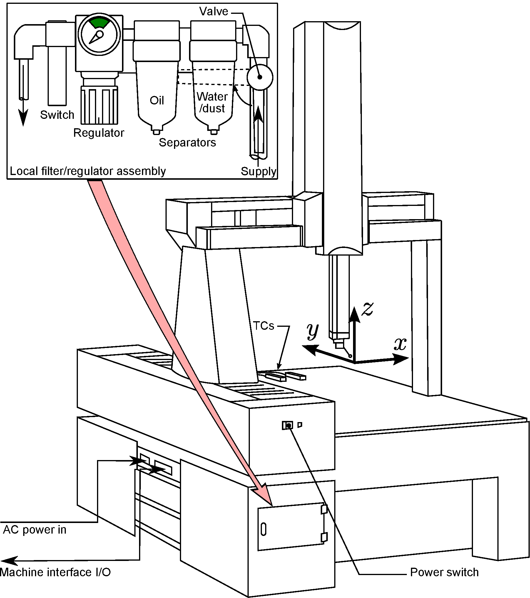
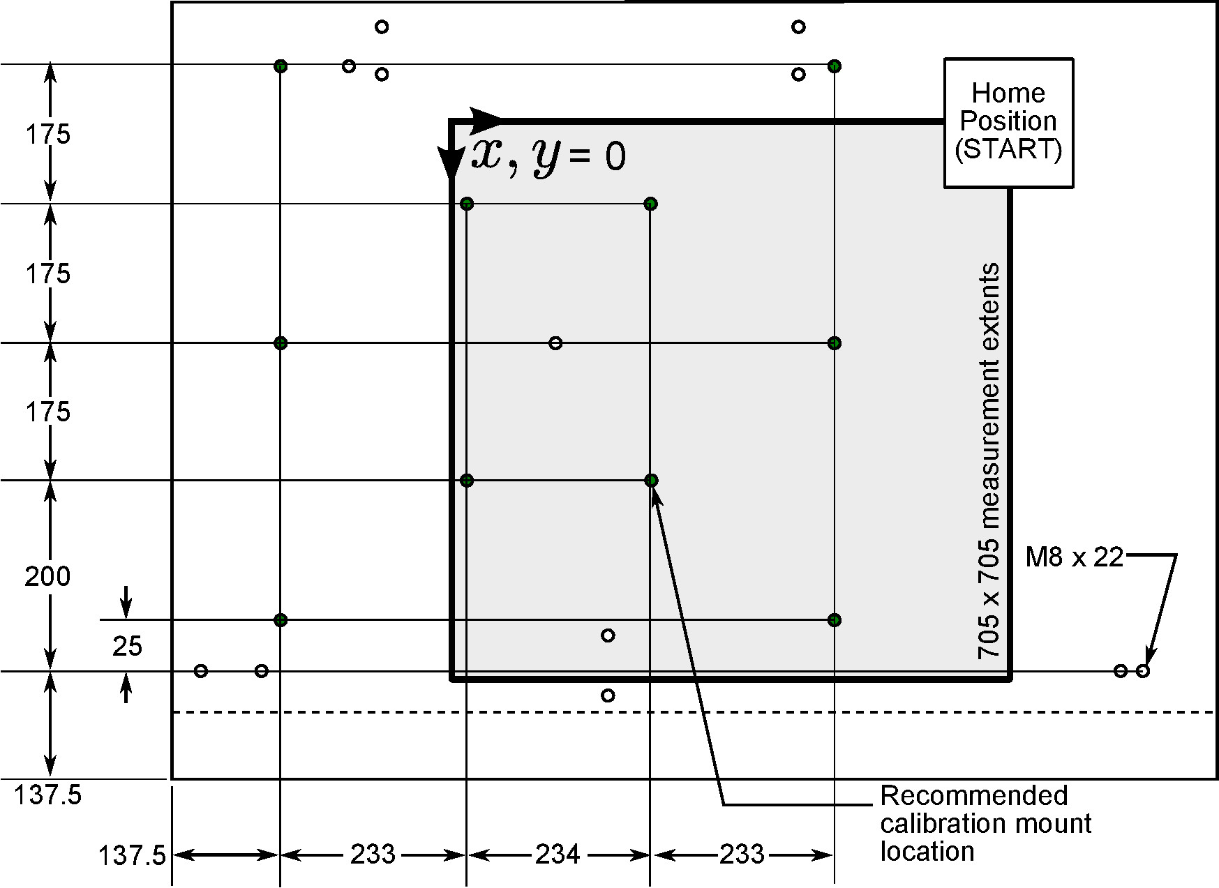
Fig. 2 details the bed dimensions and measurement capacity in the directions. According to Mitutoyo documentation, there are 9 key locations at which specimens to be measured may be mounted, with other locations either outside of the range of measurement of the machine, or are positions for further accessories such as a probe tree, calibration spheres or bed extensions. The overall weight capacity of the bed is 800 kg. Note that the bed should be treated with care as it is quite brittle. It is quite easy for the bed to be damaged by dropped specimens; special care and attention must be paid when first placing the specimen directly onto the bed and should be avoided, if possible.
1.1.2 Machine controls
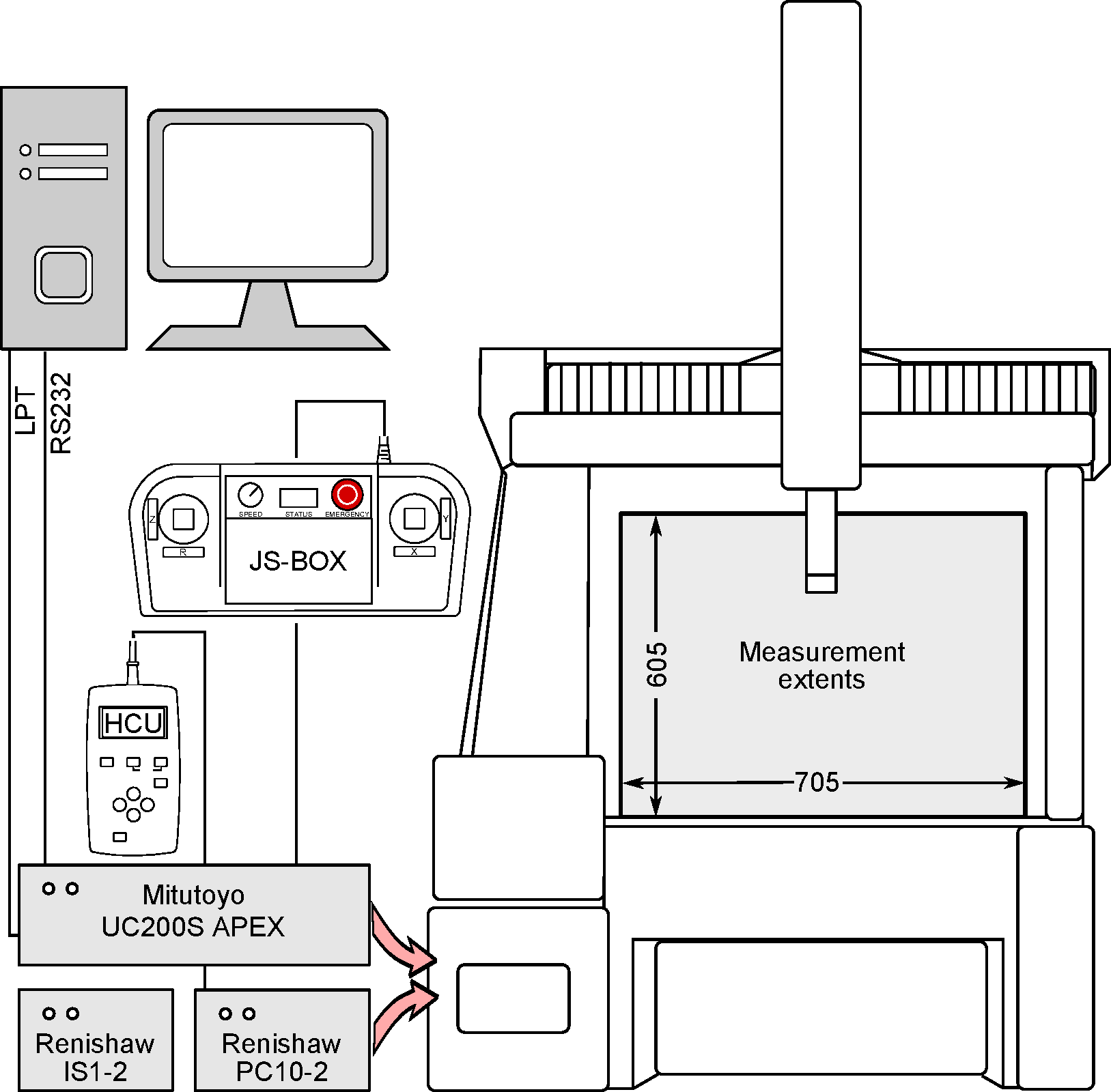
Fig. 3 shows the main controllers and measurement capacities. Beyond the main control PC, there is a Mitutoyo pendant (JS-BOX) to control the CMM, as well as a pendant (HCU1) to control the Renishaw probe. These pendants work outside of the influence of the control PC as they are connected directly to the respective driver modules. The computer communicates with the main Mitutoyo controller via a parallel (LPT) port and an RS 232 (COM) port.
The main control pendant (Fig. 4) consists of two joysticks with integrated buttons on the face and an array of soft-touch buttons contained between. There is also a 7-segment LCD display on which machine status is displayed, a feed-rate override knob and a latching emergency stop.
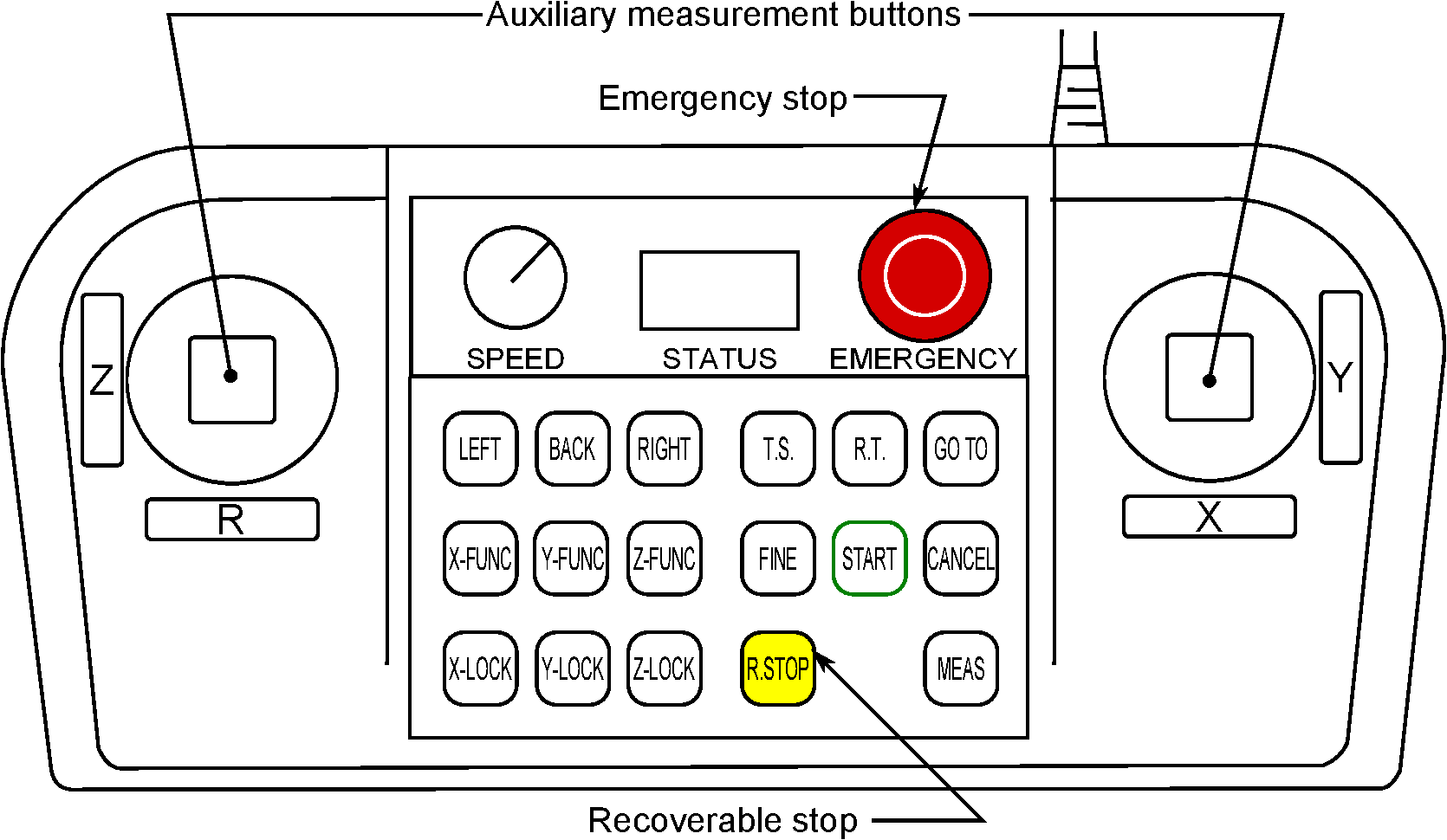
The right joystick controls movement of the machine in the and axes, (up and down, left and right, respectively) and the left joystick controls movement in the (up and down). The left joystick can also control a rotary table which the present machine is not equipped with. Both of these joysticks are analog, meaning that the further that they are depressed to their travel extents, the faster the probe will move. Additionally, the joysticks accept simultaneous input; depressing the right joystick to the north-east will enable simultaneous movement on the and axes.
The status LCD display will show machine mode, current feedrate override value and error code, depending on which mode the machine is currently under. The feedrate override knob (labelled SPEED) will allow the operator to override the movement speed which has either been pre-programmed or has returned to default values, ranging from 10-100%. While the button functions are described in detail in the Mitutoyo documentation, the most important soft-touch buttons are described in Table 1.
| Label | Description |
| START | Moves measuring head to home position (Fig. 2) |
| R. STOP | Temporary stop; machine does not need power cycling to clear error codes |
| MEAS | Places machine in measurement mode; buttons are mirrored on either joystick |
| X/Y/Z-LOCK | Filters joystick movement; e.g. X-LOCK only allows movement along |
The most important button on the pendant is the emergency stop. Depressing the emergency stop button will cause it to physically latch, and posts an error to the controller which arrests all machine function instantaneously. Clearing this error or recovering from an emergency stop is not possible without physically unlatching the emergency stop button and power cycling the machine. The recoverable stop button should not be used as a replacement or auxiliary emergency stop as some portions of the part program may still be running.
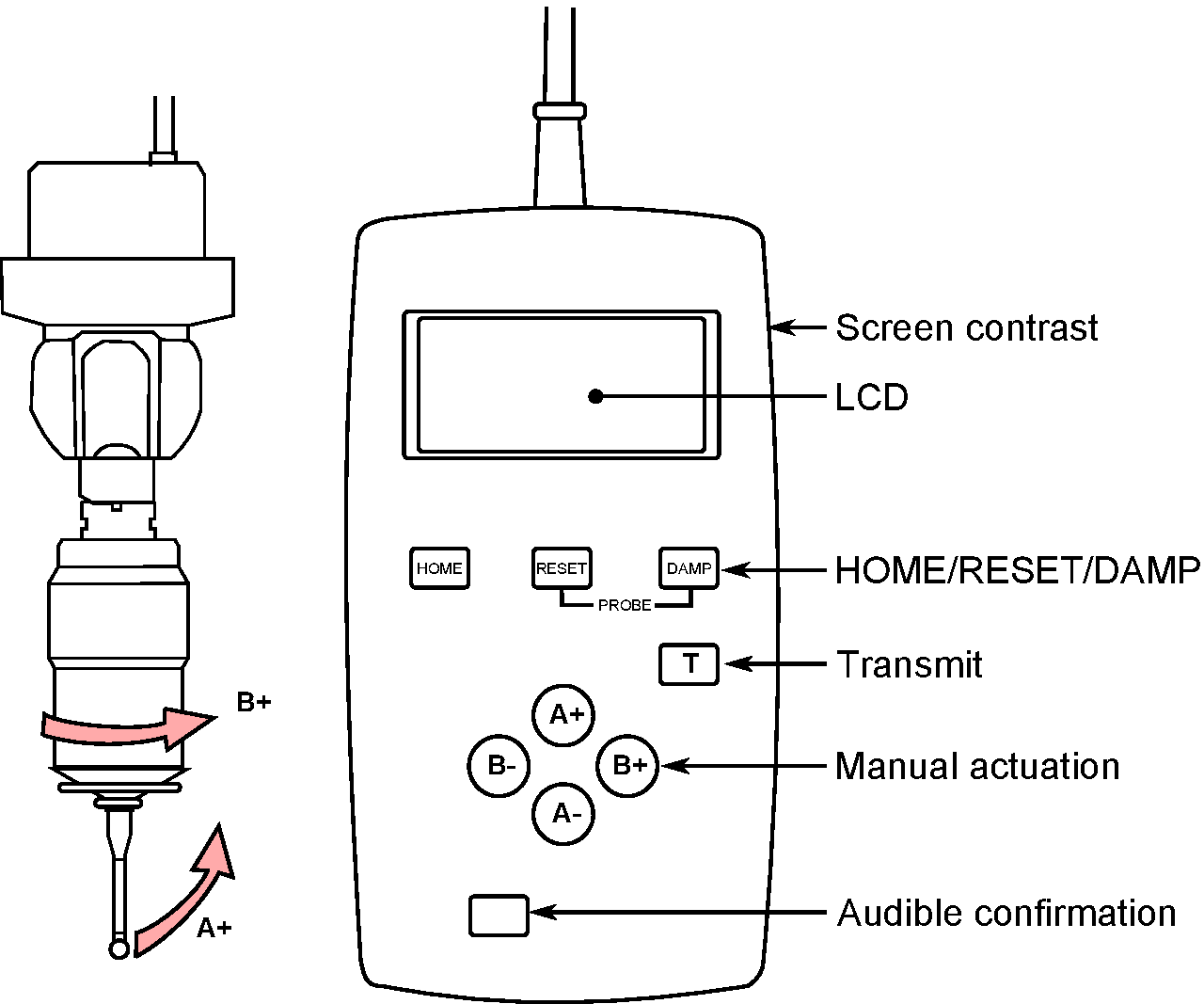
A second pendant is used for controlling the multiaxial Renishaw probe head. A depiction of the pendent is provided on Fig. 5. The principal features on this pendant are the soft keys to control probe movement (labelled ‘Manual actuation’) and the LCD screen which provide probe position, status and error codes. The A keys redirects the probe tip to incline from the axis, and the B keys cause the probe head to rotate about the axis. Each button press will move the head by 7.5 in either direction. Key presses must be serial, i.e. simultaneous movement about A and B are not possible.
1.2 Startup and shutdown sequences
There are a number of steps to follow when starting up or shutting down the CMM as there are a number of inter-related components which must initialize or be turned off sequentially.
1.2.1 Startup
- Walk around and inspect the machine for obstructions and dirt/dust on the inspection surface, inspect pneumatic traps for elevated levels of contaminants. Rectify as needed.
- Mount the specimen or calibration equipment while the machine is inactive.
- Position thermocouple probes proximate to your workpiece (if necessary).
- Ensure that there is compressed air service available and open the room’s supply valve. If the compressor has been off overnight, wait at least 15-20 minutes after the compressor has been active before opening the room’s supply valve.
- Ensure that the regulator on the room’s supply valve reads green.
- Open the valve on the machine (Fig. 1), and ensure that the regulator reads green.
- Switch power on from the wall socket to the controllers.
- Switch the CMM on by pressing the power button momentarily. Both pendant screens should provide
status output, and the Mitutoyo screen should read:
for ‘Absolute’ mode. - Power up the control PC and wait for the operating system to load. Do not start any CMM-related software.
- While the PC loads the operating system, jog the probe head clear of any components which may be
mounted on the bed with the JS-BOX pendant. Once the head is clear, stand clear of the machine and
press
START on the pendant. The machine will then move move along its axial limits back to the ‘home’ position (Fig. 2).
- Once the machine is at the
START position, the LCD display on the pendant will display the current feedrate override value. For example, if the override is set to 94%, then the screen will display:
- Once the operating system on the PC has loaded, then the respective Mitutoyo control software may be loaded.

Note that the machine will move rapidly to the axis limits, find the limit, move away, and then approach it slowly. This `limit bounce' should be accounted for when making sure that the probe is clear of all points of interference.
1.2.2 Shutdown
- Save any programmes and terminate any CMM-related software running on the control PC.
- Move the probe clear of any specimens or items mounted to the bed and approximately 50-100 mm away from the home position on all axes.
- Power down the CMM with the power switch on the front of the machine.
- Switch off power to the Mitutoyo and Renishaw driver boards.
- Power down the control PC.
- Close the valve on the CMM air manifold.
- Close the valve on the room’s air supply.
1.3 Error codes
Error codes may be reported by either the CMM or through the PC interface for a number of reasons such as
communication faults, emergency/recoverable stop events. These are reported in the form of error codes on the
pendant LCD or through the PC interface. Lamps situated on the
at CMM startup indicates that one of the joysticks was held during initialization. Similarly, if the emergency
stop is pressed, then this code will appear:
Both of these codes are ‘unrecoverable’, and require power-cycling to clear. Any code between E100 and E499
is recoverable; these include errors in communication, receipts of commands outside the capabilities of the
machine, etcetera. Any code displayed above E500 is unrecoverable.
The sequence for power cycling the CMM to clear these errors involves following shutdown steps 1 through 3, skipping step 2 if manual control is not possible. If an error is recorded at the Renishaw head, then shutdown step 4 should also be followed. Wait at least 20 seconds prior to commencing startup, whereby startup steps 7-12 (excluding 9) should be followed sequentially.
2 Part programme definition and probe designation
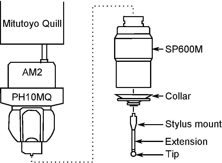
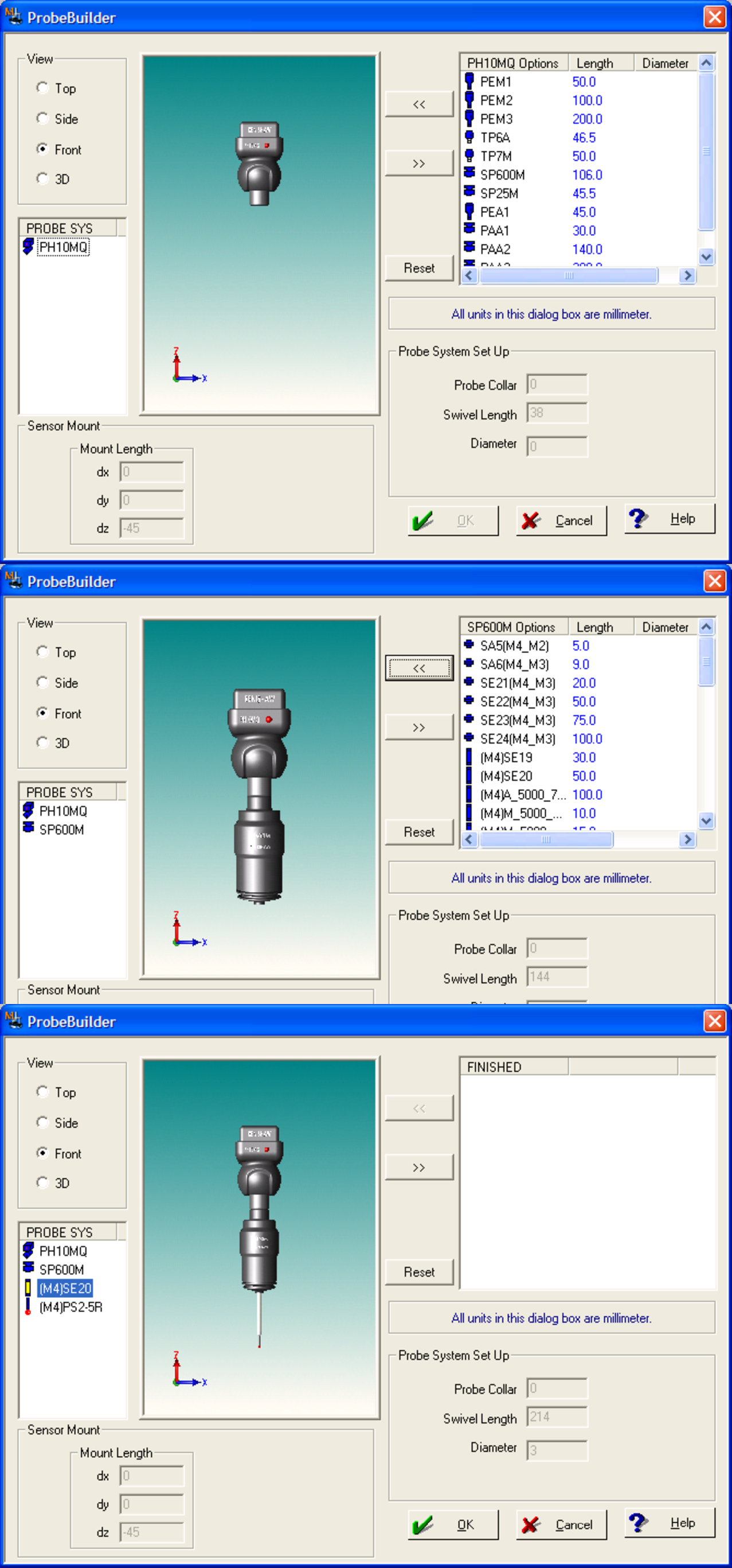
This section will describe the various physical parts comprising the Renishaw probe system, and how they are integrated into the Mitutoyo software. Fig. 6 shows the general configuration of the Renishaw system. The PH10MQ unit allows the probe tip to rotate about and around the axis, as depicted in Fig. 5; this unit is referred to as an ‘autojoint’ in Renishaw literature. The SP600M sensing probe may be connected to the autojoint, or may have another probe mounted directly instead. The SP600M allows for high speed contact measurements as any deflection in the probe tip causes an optical transducer to trip inside the probe body. After the SP600M are the stylus mount options (extensions, adapters etc.), terminating with the measurement tip. These styli mounts are connected to the SP600M with the means of a collar; this collar is designed to be used with a probe ‘autochange’ system with which the current machine is not equipped.
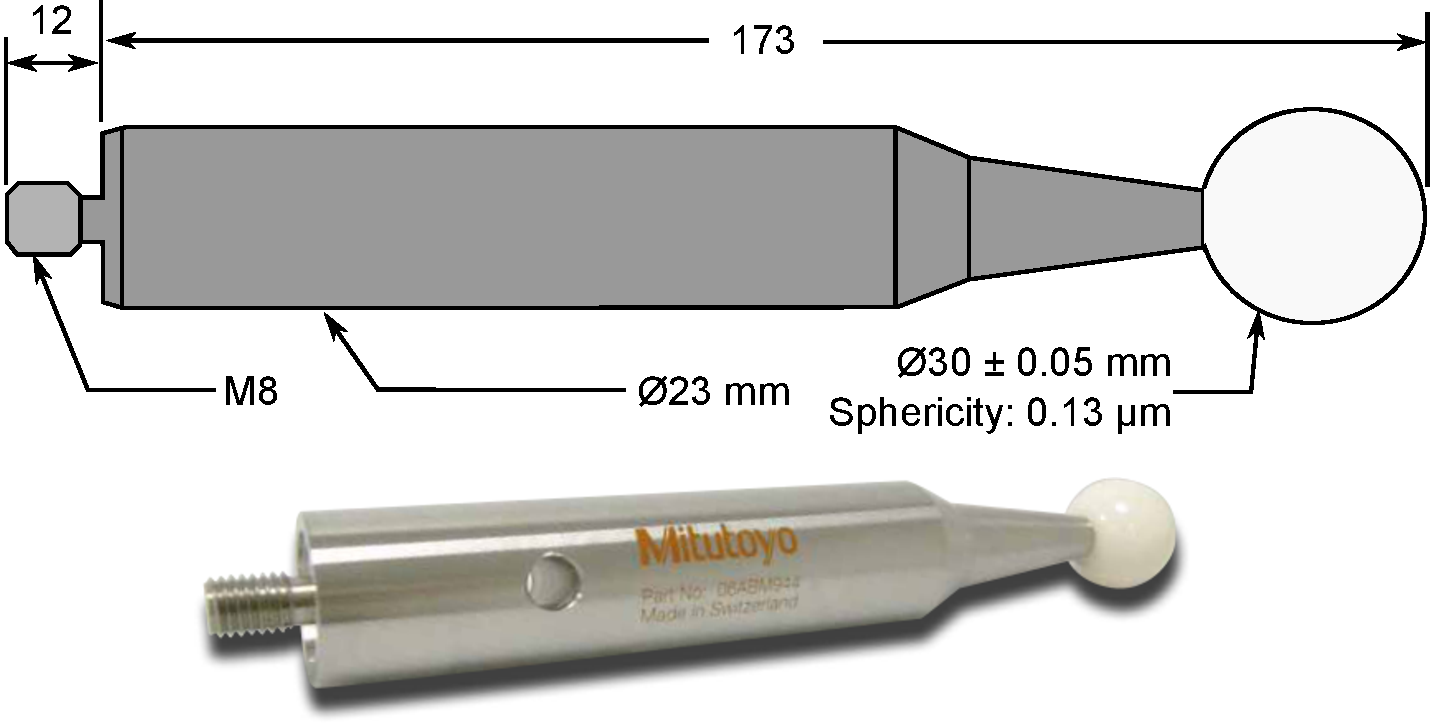
As probes configured of styli and extensions of various lengths and autojoint positions will all have different compliances and accuracies, calibration of each probe is necessary. This is accomplished with measuring a calibration sphere referred to as a ‘Masterball’ as shown in Fig. 7. The calibration sphere is usually placed at in a central location of the bed so that any probe configuration can ‘see’ it. While some industrial CMM users will leave a calibration point permanently on the bed and program around it, best practice is to remove it after each use to eliminate obstacles which may cause a crash.
Renishaw probes and styli are grouped according to the main size of thread on the final tip: they are
grouped in terms of M2, M3 and M4 threads. In order to change between different configurations, specialty
tools are required. These are small tools resembling golf tees which are required to separate the extensions
from the stylus mount and tips, and Renishaw-specific spanners and church-keys to remove the SP600M head.
Each configuration and position of the autojoint (corresponding to
2.1 Creating a new part program with MCOSMOS
The following is the sequence to create a new part program with Mitutoyo MCOSMOS CMM software and ‘build’ probes. This sequence is written from the standpoint of starting a new part programme without any pre-configured probes available.
- Start first by launching the MCOSMOS software, and select
Part Create a new part (Fig.8).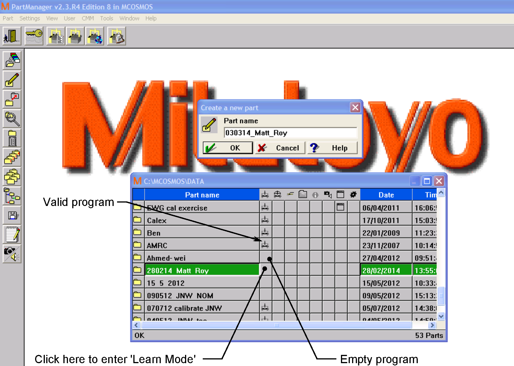
Figure 8: MCOSMOS main screen showing the ‘Create new part’ dialog, learn mode short cut to calibrate/define probes, and examples of programs with valid and empty probe definitions.
- Click on the tile beside the new part name (Fiq. 8) or select
CMM Learn mode to allow the PC control of the CMM. Do not touch the pendant(s) until the machine control window appears or else an unrecoverable error will result. Once the Machine control dialog appears as shown in Fig. 9, then the machine is receptive to both operator inputs via the pendants, as well as through the PC. - Upon launching
Learn mode , an instance of GEOPAK will also start (Fig. 9). With a new part, it is important to enter an accurate value for the material either manually or selecting one from the drop-down menu. The coefficient of thermal expansion dialog will close once a value is entered. This value will be associated with your part programme.
Figure 9: GEOPAK and Machine control dialog which appears when creating a new part programme. The thermal expansion dialog only remains visible until a value is entered. If a programme had existing commands, they would be shown in the command block segment of the GEOPAK screen.
- A new programme ‘wizard’ dialog may automatically be launched. Cancel/close this dialog.
- If there are probes predefined, that is, entries in the probe management dialog (Fig. 10), then calibration is not necessary if the existing probes accurately describe those intended for use and further programming can proceed. Otherwise, continue with the subsequent section.
2.2 Probe calibration
- Install the Mitutoyo ‘Masterball’ calibration sphere on the table - tighten by hand to avoid damage to the table inserts. The recommended position is shown in Fig. 2.
- Select
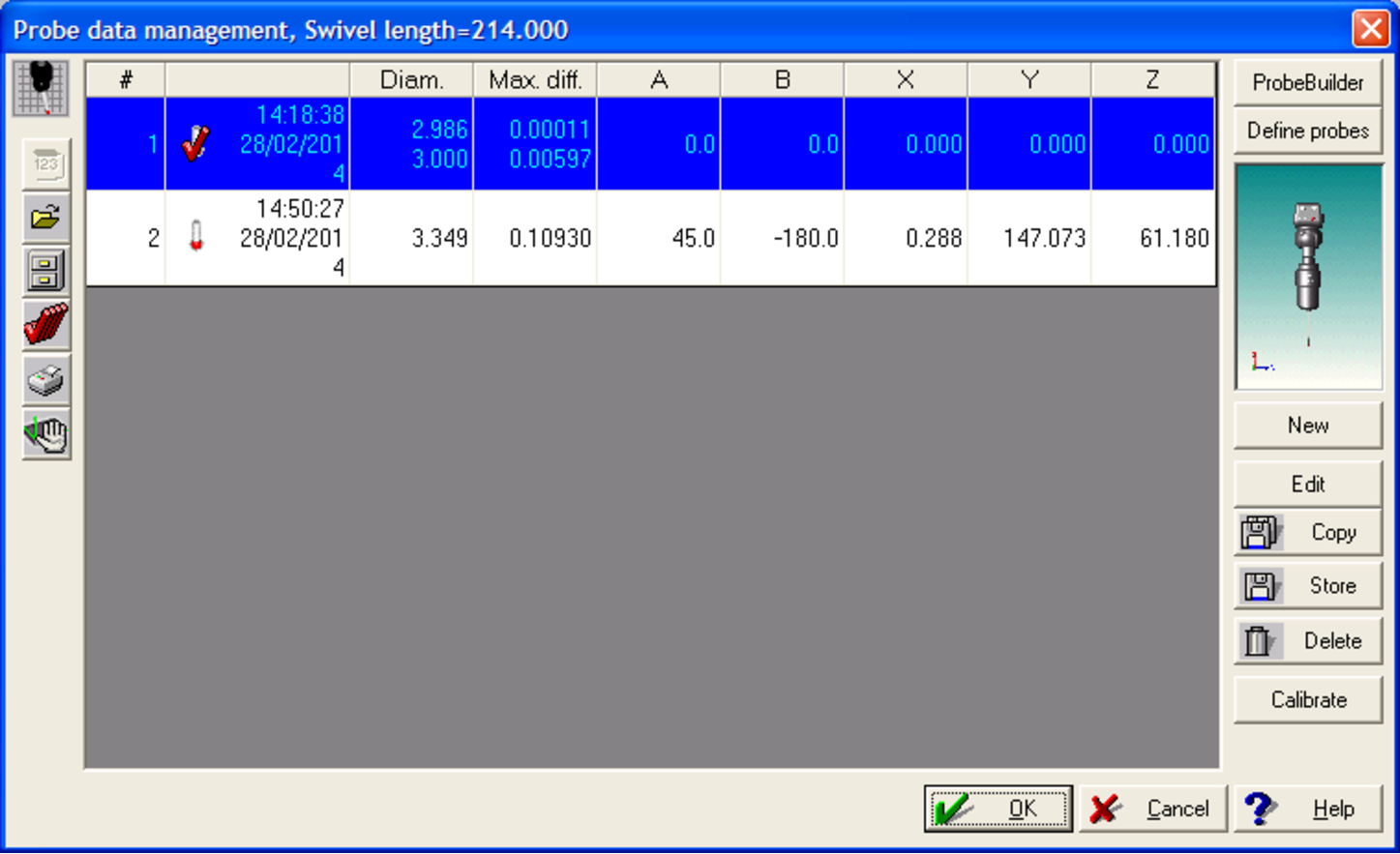
Probe Probe Data Management to access the probe management dialog (Fig. 10). In this example we will modify the second entry in the probe management dialog. TheProbeBuilder dialog is accessed by pressing the button on the top right which opens a new input screen/dialog (Fig. 11). Note that substantive changes in the probe’s configuration will invalidate the ‘calibration’ as recognized by MCOSMOS. Alternatively, a new probe can be configured by selecting’New’ and building a probe from scratch.
- Modifying/defining probes is accomplished by toggling components from the list at the right
until the entire probe is described accurately. If there is any uncertainty about any component,
measure with a set of calipers to ensure that any styli extensions and the tip diameter are
accurately described. Fig. 11 shows the three main steps starting from the autojoint (top frame)
to probe (middle frame) to extension and tip to create a ‘finished’ probe (bottom frame).
- Upon exiting the probe builder with a complete probe, the ‘New Probe’ dialog will appear (Fig.
12). Enter the values of
A andB angles, and select ‘OK’. The probe management dialog will show an uncalibrated probe (Fig. 13) with characteristics displayed in red and a pendant icon instead of a checkmark. Select the uncalibrated probe so that it is highlighted and press theCalibrate button to continue.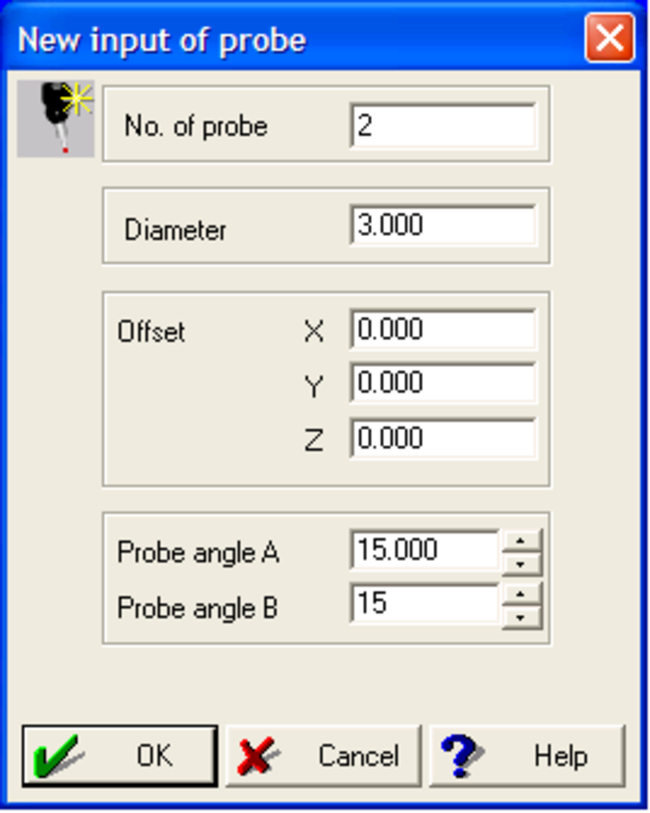
Figure 12: New probe dialog. The diameter must match that used in the probe builder step. Offsets remain at zero, and angles correspond to intended orientation of the probe tip.
- Accept the warning that the Masterball location has not been set (Fig. 14), as it will be
identified manually in subsequent steps. This will bring up the
Calibrate probe dialog , where the Masterball diameter, probe number and number of points to be employed in the calibration are all entered. The more measurement points employed result in a more accurate calibration. Selecting ‘OK’ will bring up a warning that the machine will move the probe from the current location to some new location. Ensure there is ample space for the tip to move unobstructed by jogging the probe with the pendant.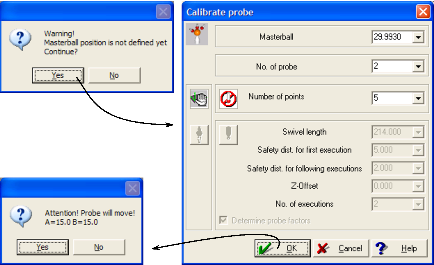
Figure 14: Intermediate calibration dialogs. The Masterball position warning appears first, followed by the calibrate probe dialog. In this dialog, the Masterball diameter, probe number and number of points to be employed are all set here. The default number of points is five. Once this dialog has been completed, then a warning will appear. Ensure that the probe tip can move unobstructed to the angular position indicated.
- Once the number of calibration points has been selected, then the
Calibrate probe screen will change to indicate that the CMM is ready to receive the calibration points from the Masterball (Fig. 15). Using the pendant, move the probe close to the measurement ball, and then pressMEAS or equivalent joystick buttons (Fig. 4) such that the LCD screen on the pendant reads:
which indicates that the CMM is in measurement mode.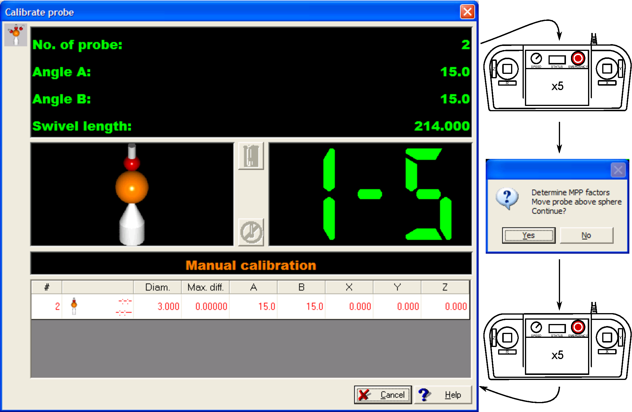
Figure 15: Calibrate probe dialog showing point entry display. The main screen (left) shows that the PC is waiting for the first measurement point on the Masterball to be performed of five. Once five points have been entered with the CMM, the MPP factors will be automatically found by scanning the ball with the stylus. Five more measurement points are required after the MPP calibration completes.
- Bring the probe tip into contact with the Masterball until an audible beep is heard. Repeat this process
until all points indicated in the
Calibrate probe dialog are satisfied. Measurement mode can be cancelled by pressingMEAS or equivalent again so that the probe can be moved rapidly between points. The best practice is to place the machine in measurement mode when moving the probe tip within 20 mm of the Masterball. - Once the points have been measured, a dialog will appear instructing the user to move the probe tip to
some point above the Masterball. Doing so and pressing ‘Yes’ will launch a diagnostic routine where the
machine
will move automatically to determine scanning factors. Selecting ‘No’ will end the calibration routine, and the probe may be used. However, line scans may not be available with the probe or may be inaccurate. Best practice is to run the MPP calibration. If the MPP calibration routine fails due to a collision, then it is not advisable to use this probe for line scanning. - At the conclusion of the MPP calibration, repeat step 7 to conclude the probe calibration.

The machine must be in measurement mode as described above to perform a measurement, otherwise it will be registered as a crash. Furthermore, contacting the probe with a rigid surface at anything more than measurement speed will damage the machine.
Once calibration has been successfully completed, the GEOPAK interface will resume whereby the user can either define and calibrate a new probe, or continue programming. Note that once a probe has been calibrated, it may be employed in any program and does not have to be calibrated prior to use. Calibration is necessary after either a long time period of disuse, abrupt changes in weather, crashes or anything else that the operator suspects may detract from accuracy.
3 Part programming
This section will outline how to generate a part programme that contains one or more contour measurements using the Renishaw SP600M scanning head with GEOPAK in ‘Learn Mode’. This section will also cover how to run a saved program, and how to make modifications to existing programmes.
This preliminary program will encompass creating three measurement elements with the subject being a pair of toe clamps (Fig. 16):
- A plane defined by three points;
- A contour scan in the plane;
- A contour scan in the plane.

The programming sequence consists of a large number of graphical interfaces within GEOPAK. Final
entries to these dialogs result in machine movement conforming to the input. Due care and attention must be
paid when programming the CMM as errors in either input or probe position may result in a crash. Good
programming procedure is to turn down the feed-rate override on the pendant to 10 after every program entry,
and advancing the speed to ensure that the machine is moving as intended. Furthermore, the operator
should have the pendant in hand and ready to press
When building a program for the first time, be prepared for the machine to move unpredictably. Turn down the feedrate override and be ready to either press

This button is located to the left of the main GEOPAK interface.
3.1 Creating a part programme
- If not done so already, start MCOSMOS and and select
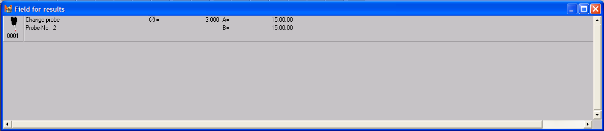
Part Create a new part (Fig.8), and follow the steps in Section 2.1 as required. - The first command in the program will be a probe change to a pre-defined probe. This
command is located under
Probe Change probe . The ‘Field for results’ dialog will update with the command after it has been executed (Fig. 17). If the specified probe is different that the one currently active, a warning message will appear informing the operator that the probe will move. Ensure that there is no point of interference for the probe.
- Any number and combination of construction geometry or ‘elements’ can be programmed once a probe
has been selected. These are accessible through the
Element dropdown menu, or via the icons at the top of the GEOPAK interface:
These icons range from a single point on the immediate left, to a contour on the immediate right. Each provides the ability to define various geometric entities based on single or multiple points. As a demonstration, click the plane icon or
Element Element Plane . - The element plane dialog will appear with a multitude of options (Fig. 18). Here, define a plane
with three measurement points, calculating the plane by interpolating between the points. The
‘Memory’ input dictates the number that the plane will appear in memory (i.e. the plane is
number 1 of a larger number of element planes). Use the default measurement point ‘Type of
construction’, and ensure that the auto-calculate button is depressed.
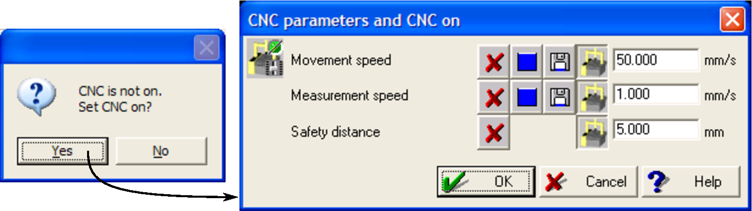
- Upon hitting ‘OK’ for the element plane, a warning that ‘CNC is not on’ (Fig. 19) will appear. This
merely states that the GEOPAK is running passively when communicating with the CMM, and is asking
whether the ability to send the machine commands via Computer Numeric Control (CNC) should be
activated. Accepting the warning will bring up the CNC parameter window. These CNC operating
parameters are summarized in Table 2.
Table 2: CNC parametersParameterDescriptionRecommended to maximum values Movement speed Probe movement speed between measurements
50-200 mm/s Measurement speed Probe movement speed when finding a surface
1-3 mm/s Safety distance Retraction distance along from the surface after making a measurement
5-0.5 mm
- Once the CNC parameters have been set, then GEOPAK will wait for measurement points with a display
similar to that in Fig. 20. Note that the ‘Field for results’ pane has been updated to include a ‘CNC on’
command to account for setting the parameters earlier. The next step is to measure three points to define
the plane. Measure the bed at the three points indicated in Fig. 16 to be entered in the same manner as
described in the previous section: using the pendant, move the probe close to the measurement point,
and then press
MEAS or equivalent joystick buttons (Fig. 4) such that the LCD screen on the pendant reads:
which indicates that the CMM is in measurement mode. In order to ensure that the probe moves in a single axis at a time, one may use theX/Y-LOCK function to temporarily disable movement in the respective direction.
Figure 20: GEOPAK screen waiting for operator input. Under the ‘Measurement Display’ pane, the element currently being measured is shown on the left. The current and total number of points needed are shown on the right. The format ‘1-3’ infers that measurement of the element in question is on point one of three.
- Once the three points are entered, then GEOPAK updates with entries in the ‘Field for results’,
‘Graphics of elements’ and ‘List of elements’ (Fig. 21). A new element can be now programmed, or, if a
mistake was made in entering data, this latest program can be deleted by entering
Program Delete last step . This will remove the command from the ‘Field for results’, and permit a new command to be entered in its stead, or re-definition of a measurement element.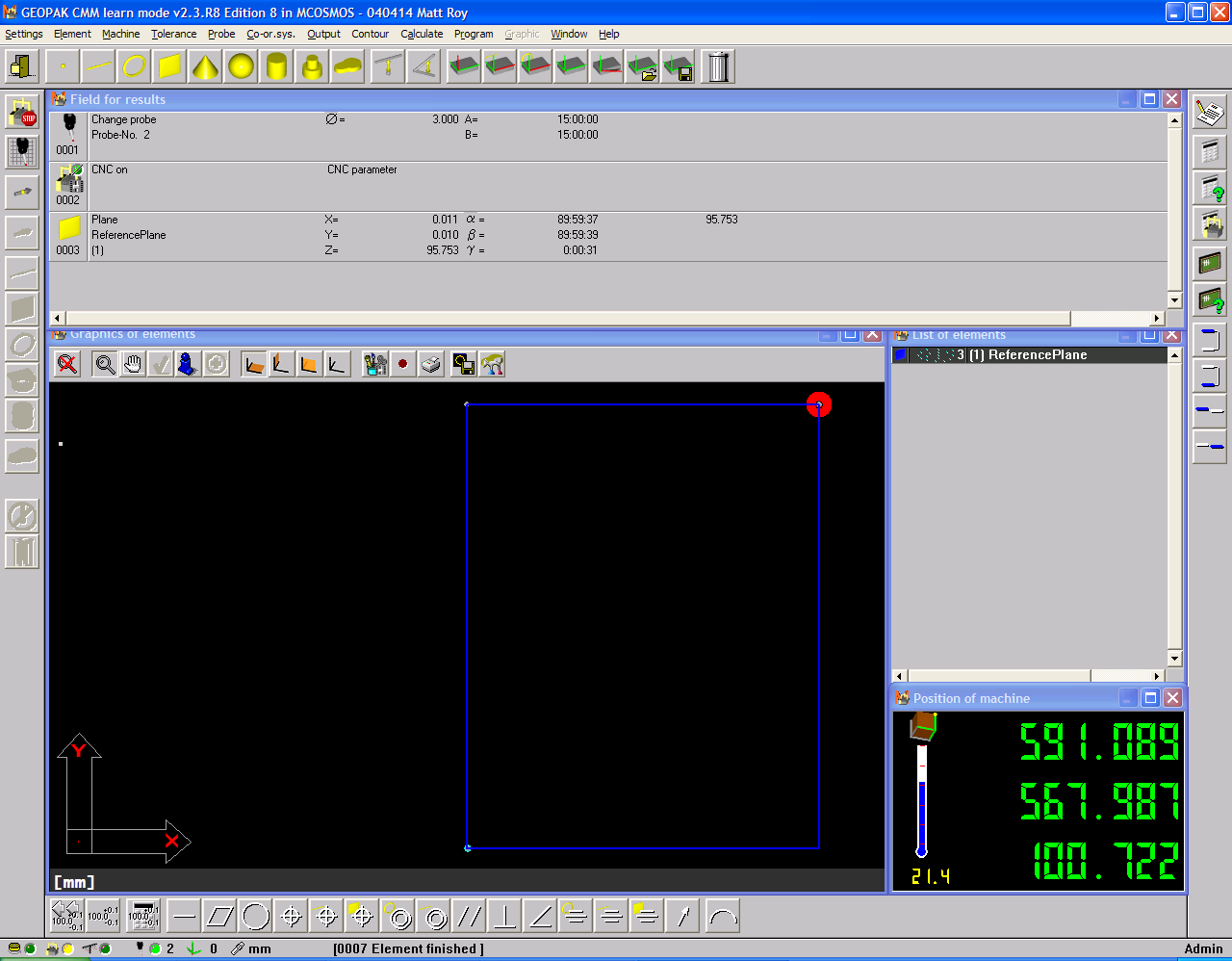
Figure 21: Completed plane element in GEOPAK. ‘Field for results’, ‘Graphics of elements’ and ‘List of elements’ have all been updated.
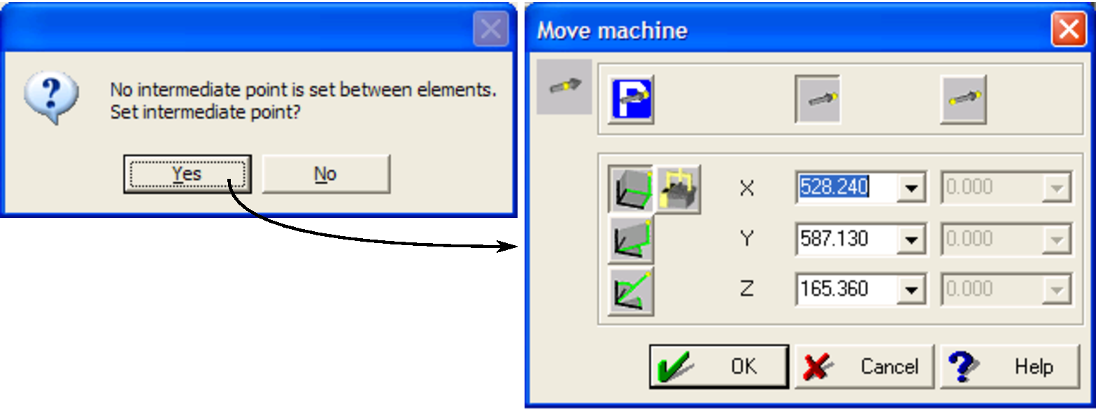
- Next, the
contour element will be programmed. Select either the contour icon or
Element Contour . GEOPAK should provide a warning that no intermediate point was set for the probe to move to prior to starting the measurement of a new element (Fig. 22). Acknowledge the message to bring up the ‘Move machine’ dialog. This dialog is also available throughMachine Move machine , to pre-empt this warning message. Move the machine to an appropriate point with the pendent, and capture this position by pressing the current position icon in the ‘Move machine’ dialog:

and then pressing ‘OK’.
- Once the intermediate point has been programmed, then the element contour dialog should appear (Fig.
23). Name the plane, and ensure that the definition and auto-calculate options are selected as for the
plane element (Fig. 18).
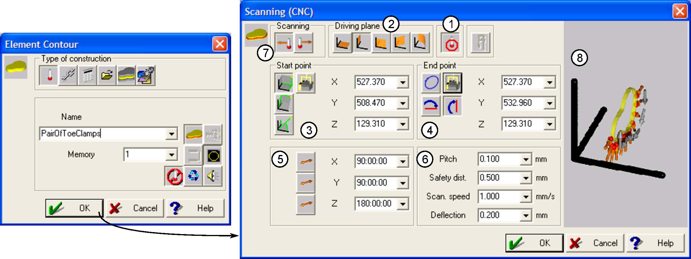
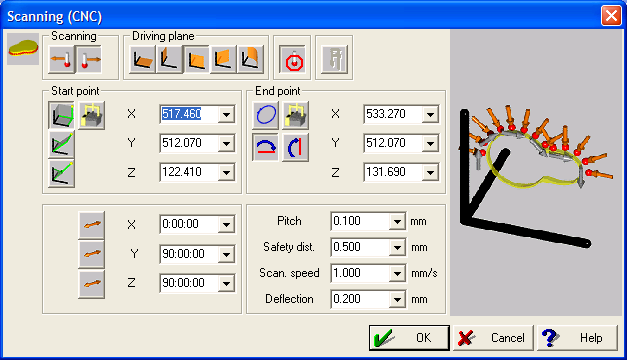
Figure 23: Dialogs to create new contour element in GEOPAK. The ‘Scanning (CNC)’ settings shown in this dialog produced the first scan depicted in Fig. 16.
- Once the contour dialog has been acknowledged, then the ‘Scanning (CNC)’ dialog is brought up. With
this interface, all of the characteristics of the contour scan are entered, described according to the labels
on Fig. 23. These are summarized in Table 3. The detailed steps to follow in order to generate the first
scan as shown in Fig. 16 are:
- Ensure that probe calibration is active.
- Set the driving plane to be the .
- Manually move the probe to a site proximate to where the scan should start, and populate the coordinate inputs using the ‘current position’ icon (Table 3).
- Set the end point by moving the probe to a site proximate to the end of the scan. Populate the coordinate inputs the same way as the start point. Ensure that the ‘Ignore second axis’ icon is selected, so that the scan will terminate when the probe arrives at the coordinate.
- Enter 180:00:00 for the
Z driving axis. This will bring the probe down to approach on the axis to find the surface. - Set scan parameters. Note that the
Deflection value is not fully documented. - Reverse the scanning direction such that the probe moves along the positive
axis, otherwise it will move in the negative
direction due to the
Z driving axis being flipped 180.
Table 3: Contour scanning inputs. Item numbers correspond to Fig. 23.Item Description 1 Probe compensation: this adjusts for running a round probe tip inside corners with radii smaller than the probe tip. This is recommended to be always on.2 Driving planes: Can be either cartesian, cylindrical or polar. Cartesian planes are relatively straightforward, and match absolute orientations. For the more advance driving planes or if an origin/axis shift has been programmed, refer to the GEOPAK documentation for appropriate settings.3 Start point: Inputs refer to where the probe will start scanning from. This point can be entered manually, or the probe may be driven to the point in question and populated with the current position icon.4 End point: Dialog indicates how the scan will terminate. The circular icon indicates that a closed contour is intended. In this case, the scan will terminate when arriving at the start point. Otherwise, setting the end point for can be set in the same manner as the start point. The ignore axes icons:

will dictate how the scan is terminated for an open-ended contour.
5 Driving axes: Indicates the orientation of the scan related to the preview in (8).6 Scan parameters:- Pitch: dictates the number of points which will be measured over the scan length.
- Safety distance: indicates how far the probe will retract from the surface once the scan is complete.
- Scan speed: how fast the scan will proceed; must be in the range of 1-20 mm/s.
- Deflection: how much the probe should deflect before a point is measured.
7 Scan direction: either accepts the scan direction in (8) being accurate and ‘forward’ scanning is selected. ‘Reverse’ scanning reverses the direction depicted in (8).8 Scan preview: Shows the direction of the scan with grey arrows and measurement points in orange.
GEOPAK documentation does not thoroughly explain this point - it is assumed that having this value as small as possible for smooth surfaces will provide the greatest accuracy.
- Move the probe manually away from the part prior to pressing ‘OK’. Turn down the feedrate and be
ready to press
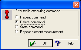
R. STOP to abort movement. ‘OK’ will cause the machine to move immediately from its current position to the start point entered in the scanning dialog. Ensure that the probe both finds the surface in question, is scanning in the correct direction and terminates the scan appropriately. Errors in entering the appropriate scanning direction, driving plane, local coordinate translations make configuring the probe to move in the correct direction challenging. If the probe is not moving correctly, pressR. STOP on the pendant or the stop icon in GEOPAK to abort movement.Stopping scanning with a recoverable stop will cause an error dialog to appear on both the pendant and the GEOPAK interface. Clearing this error dialog will produce the dialog depicted in Fig. 24. Click the ‘Delete command’ radio button and OK. It will be necessary to select
Program Delete last step a number of times in order to be able to redefine the contour element measurement.The best practice to pursue if the machine is not behaving as intended to make single changes and run again.
- Once the scan in the
plane has been completed, create a new scan to reflect the second path in Fig. 16, initiating
the contour in a similar manner to that outlined in step 8. Note that the ‘Memory’ entry in
the ‘Element Contour’ dialog will automatically increment to account for this being the
second scan programmed. Fig. 25 shows the parameters input to perform this scan. Principal
changes include new start and end points, driving plane, scanning direction and
Z driving axis.
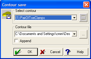
- Now that the contours have been performed, they can be saved by entering a ‘Contour save’ step, accessed through
Contour Contour save (Fig. 26). In this dialog, the location and contour or memory number are assigned. Multiple contours can be written to the same file by selecting ‘Append’.
- Once the contour save step has been completed, then the text file in the proscribed location will have the format of:
which is of the form , and coordinates.
+0528.2205 +0505.5326 +0125.6893
+0528.2248 +0505.6027 +0125.6921
+0528.2208 +0505.6605 +0125.6935
+0528.2244 +0505.7674 +0125.6920
+0528.2250 +0505.8980 +0125.6954
+0528.2237 +0505.9770 +0125.6974
+0528.2229 +0506.0406 +0125.6973
+0528.2261 +0506.1459 +0125.6948
+0528.2200 +0506.2638 +0125.6952
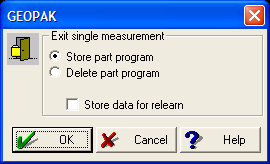
- Now that all programming steps are implemented, exit GEOPAK. Here, the option to save the program will appear (Fig. 27). Check the ‘Store data for relearn’ if you wish to modify any of the existing program in GEOPAK’s ‘Learn mode’ as opposed to the programme editor. Selecting OK will return the user to the MCOSMOS main screen (Fig. 8).

3.2 Running existing part programmes
Program completed in the previous section can be run from MCOSMOS at any time. Steps to run the programme are detailed subsequently.
- On the list of programmes in the part manager window, click on the ‘Valid program’ icon beside the programme name as shown in Fig. 8.
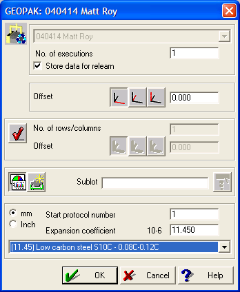
- GEOPAK in ‘repeat mode’ will launch, and a screen similar to that shown in Fig. 28 which will
allow offsets, number of executions, run characteristics, units and CTE factors to change prior
to program execution.
- Pressing OK will start the program and the machine will run through all of the operations
previously programmed. It is important to turn down the feedrate override and watch the
machine for the first time when running a new program to check for unanticipated collisions. At
the program’s conclusion, a screen similar to the one shown in Fig. 29
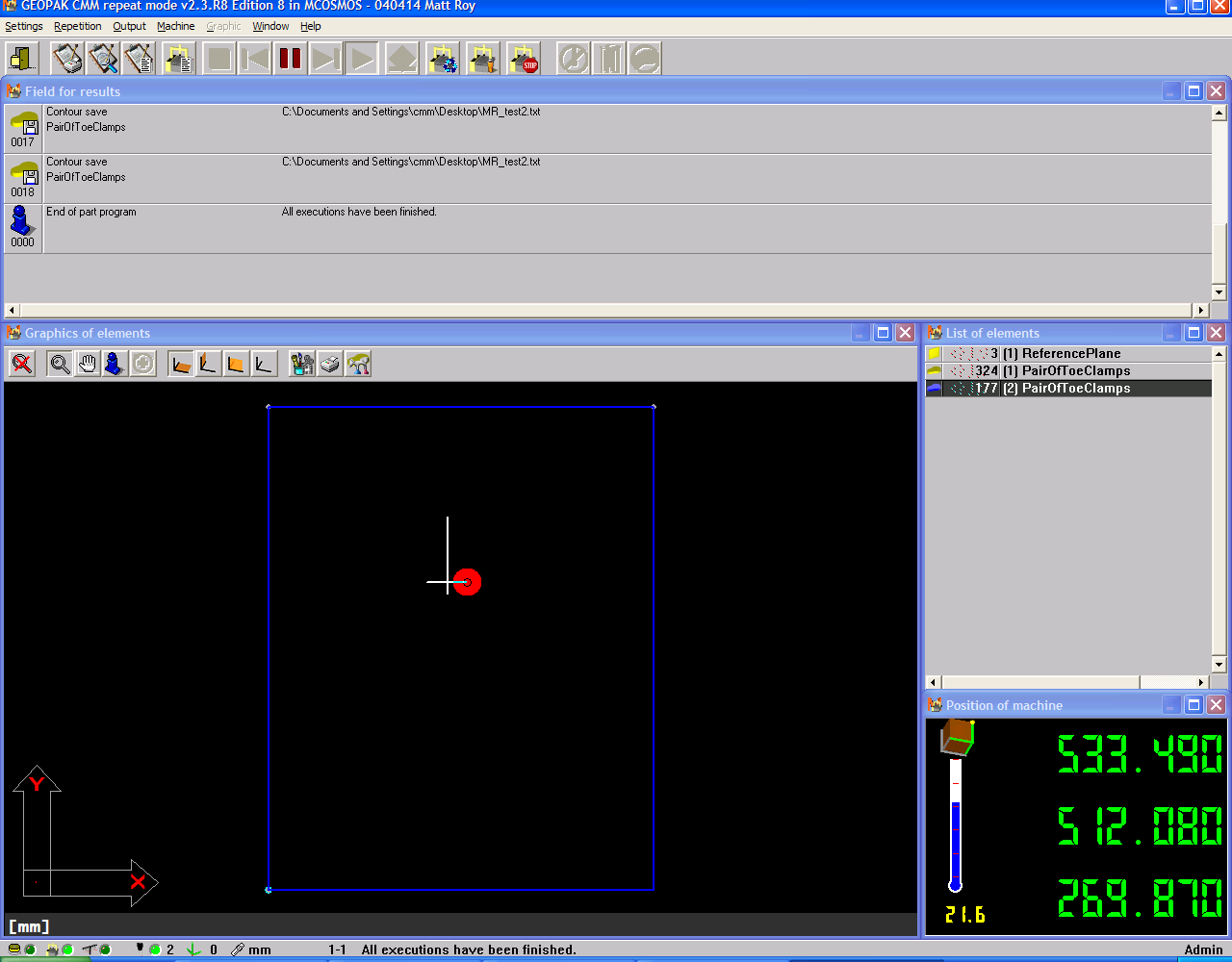
Figure 29: GEOPAK screen showing a completed program. The ‘Graphics of elements’ pane shows the measured plane element in blue, the two contour measurements are shown in white and the current position in red.
- In order to leave ‘repeat mode’ to add further operation to the existing program, press the relearn icon at
the top of the interface:

This will permit the operator to add to the programme if the ‘Store data for relearn’ option was not selected when the program was originally saved. If the option was selected, then it is possible to both add to or edit the existing operations comprising the programme.
4 Summary
This concludes the basic guide on how to generate basic measurements with the Mitutoyo Crysta-Apex 776 in learn mode. For highly repetitive measurements, the likes of which that are used when performing profilometry in practice of the contour method, almost all probe movements can be scripted and imported using the ASCII-GEOPAK conversion module. However, it is important that the user understands how the machine is programmed manually first before trying out measurement programmes developed programmatically.